The AMSU instrument detects earth/atmosphere emitted radiation in the microwave portion of the electromagnetic spectrum. Microwaves, in comparison to more familiar infrared or visible radiation, are less energetic and have longer wavelengths (distance between successive wave crests/troughs) on the order of centimeters (10-2 meters) vs. micrometers (10-6 meters). Based on energy considerations and AMSU-A instrument performance, this dictates that the sensor be placed in a lower earth-orbit (~810km above the earth's surface vs. ~36,000km for geostationary satellites) to improve instrument signal-to-noise. The AMSU-A (temperature sounder), a 15 channel passive radiometer, detects energy emitted by atmospheric molecular oxygen (a major atmospheric constituent) and is largely unaffected by the presence of clouds--from the emission source, through the atmosphere, to the sensor which resides on the NOAA-15-19 polar orbiting satellites as well as the NASA Aqua, EUMETSAT METOP A/B and China FY-series satellites.
AMSU-A Sensor and Radiative Transfer Theory
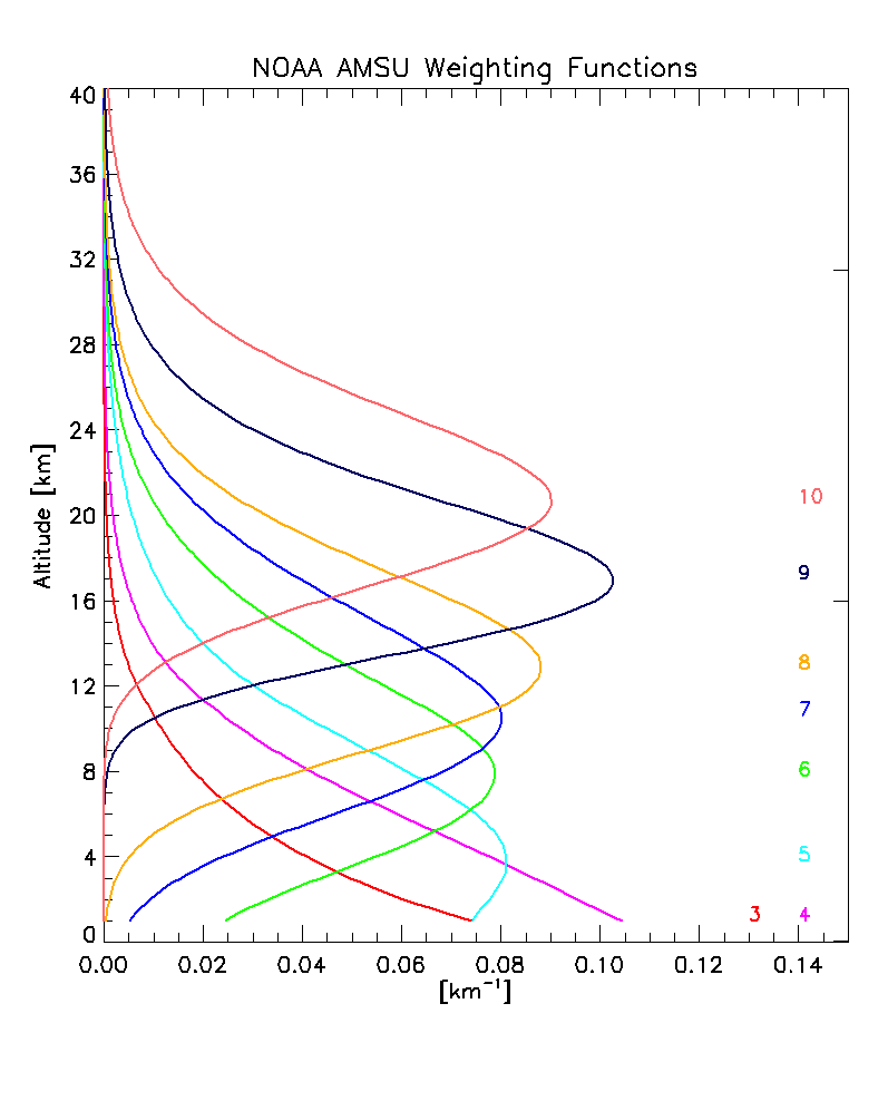
Contributions to the upwelling terrestrial radiation sensed by the AMSU-A (neglecting the effects of reflection and scattering which themselves can behave as source/sink terms) are largely comprised of two terms--the earth's surface and the overlying atmosphere. Individual AMSU-A channels (i.e., frequencies) are carefully chosen based on principles of radiative transfer theory. Each channel (frequency) is radiatively selective in the sense that it detects microwave radiation from discrete layers within the earth's atmosphere. Satellite meteorologists typically relate the radiation sensed in individual AMSU-A channels/frequencies to specific atmospheric layers (characterised by the abundance of molecular oxygen O2 and temperature) by use of a term called a weighting function:
Exploitation of AMSU-A Channels 5-8:
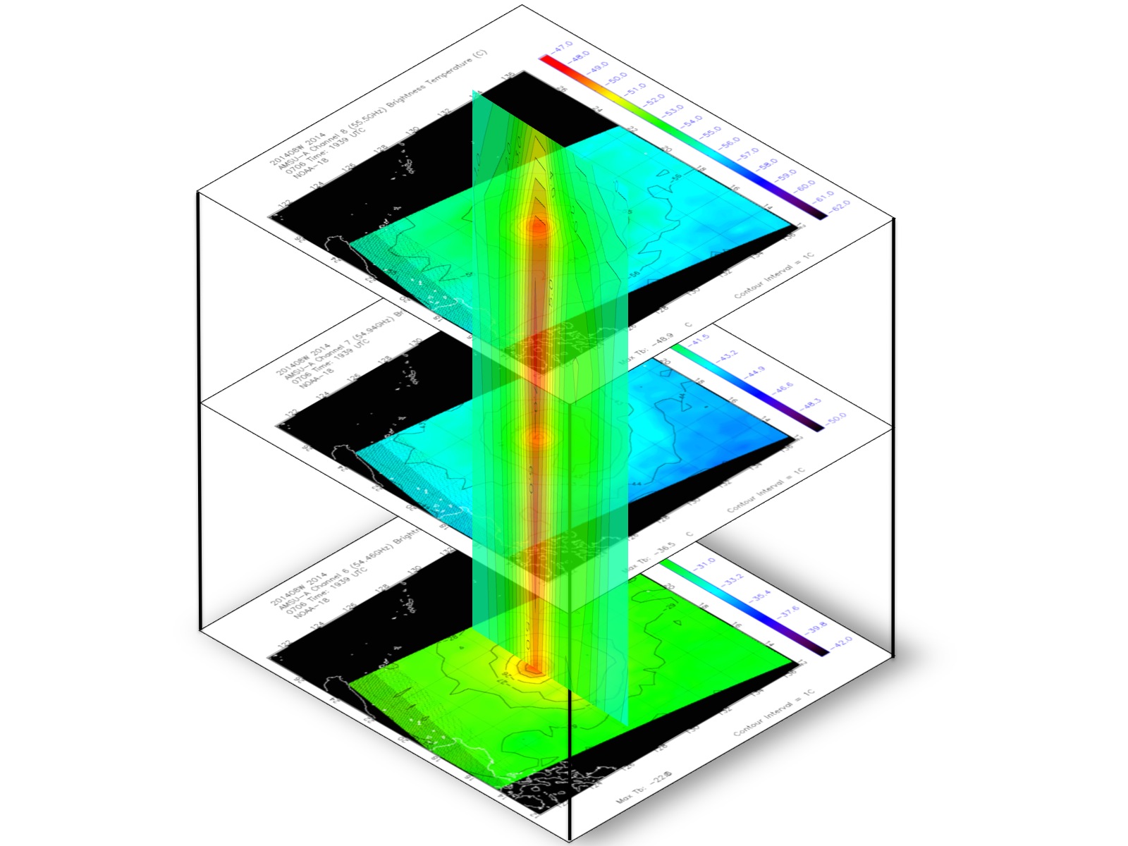
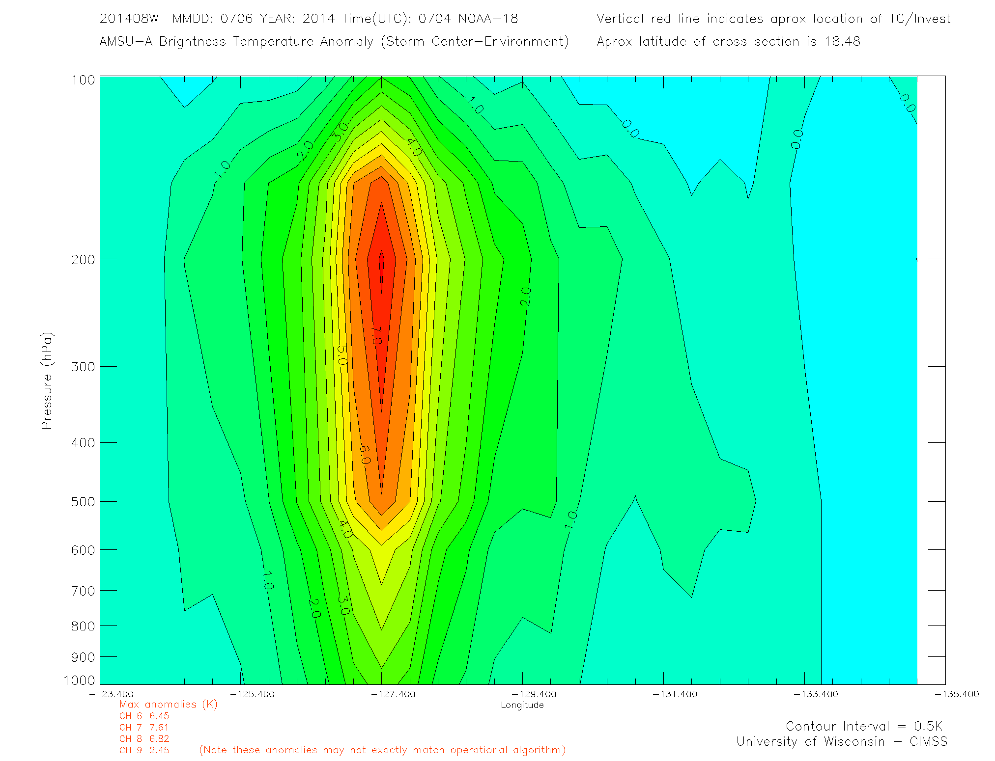
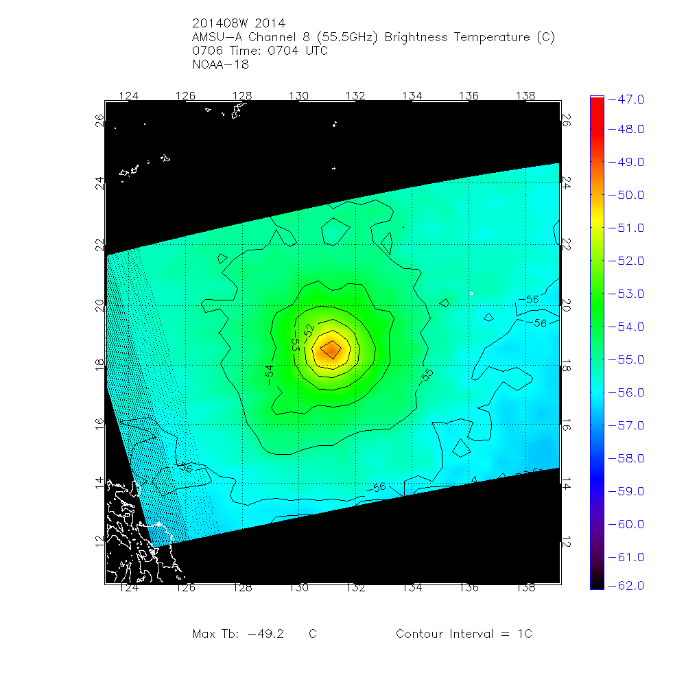
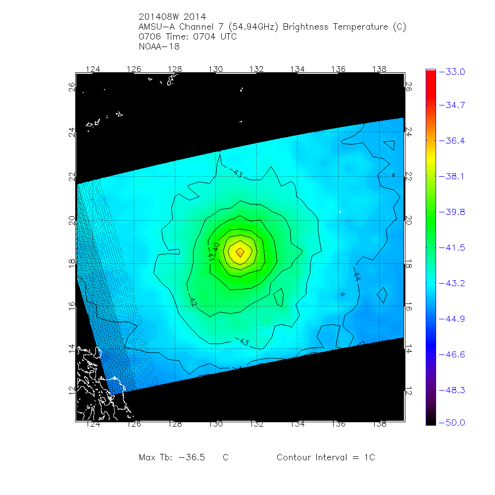
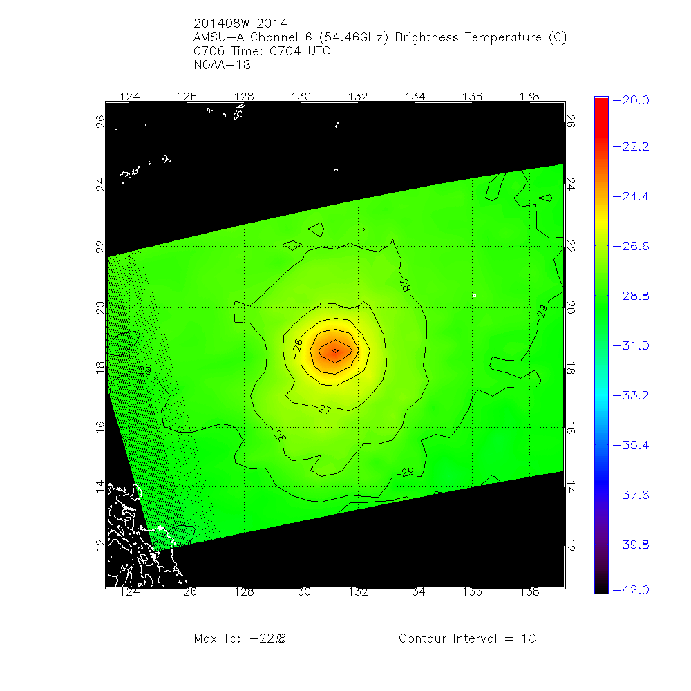
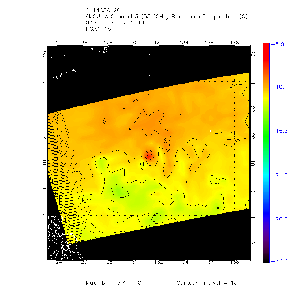
As tropical storms develop into hurricanes, they're characterized by upper tropospheric warming (the troposphere being defined as that portion of the earth's atmosphere extending from the earth's surface to approximately 15km altitude) as a result of adiabatic warming/compression of air as it subsides (sinks) within the storm center. The following is an example of a cross-section image of Typhoon Neoguri 2014 derived from AMSU-A data (contours are degrees C above storm environmental temperature):
A similar, more familiar, warming occurs when inflating a bicycle tire with a hand held-pump. Within the sealed pump cylinder, air is compressed and warms. The result is a bicycle pump that becomes warm to the touch. Subsidence within a tropical storm/hurricane warms the overlying troposphere, suppressing clouds and leads to the characteristic 'eye' commonly observed in satellite pictures.
AMSU-A Channels 5-8, as visualized on the UW-CIMSS AMSU Homepage during tropical storm/hurricane events,As storms mature and the circulation/associated convection become more organized, the amount of microwave radiation emitted by the atmosphere towards the AMSU-A instrument increases as tropospheric temperatures (again, as a result of storm-related subsidence/warm ing) increase. The exception occurs in cases where ice/liquid water droplets reduces the upwelling radiation due to the effects of scattering (commonly seen in AMSU-A Channel 5).
The matrix of AMSU-A brightness temperatures (analogous to temperature) generated for each storm system shows the time evolution
(from left to right) as well as the vertical distribution of storm-related tropospheric heating (top to bottom). In general as
the storm becomes more intense the warm anomaly seen in the images will increase in magnitude. This is best seen in channels
7 and 8 which are high enough to not be affected by precipitation. In storms with very large eyes or storms which have lost much
of their convection strong warming may be present in channels 6 and 5. An example of the imagery for Typhoon Neguri (2014) is below. Neoguri was estimated to have winds of 120 knots with a pressure of 930 millibars at the time of these images :
| Channel | Latest Data |
 100 hPa |
 |
 200 hPa |
 |
 350 hPa |
 |
 550 hPa |
 |
| AMSU-B 89 GHz |
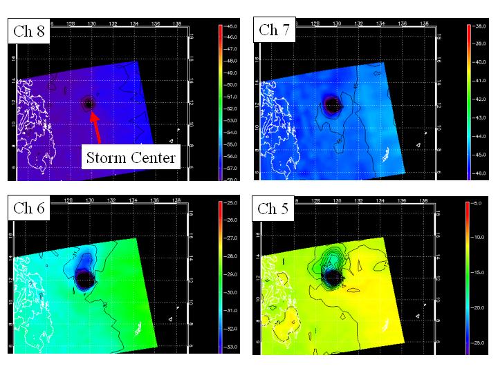
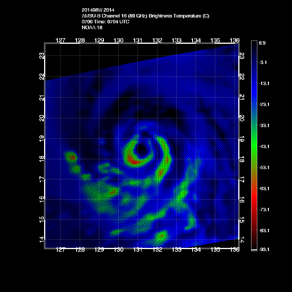 |
Notice that a warm anomaly can be seen in all 4 channels extending from channel 8 down into channel 5. However in channel 5 the effects of precipitation in the form of cooler brightness temperatures (green shading) can be seen to the south of the warm anomaly (orange shading). This cooling corresponds well with convective banding on the south side of Neoguri as seen in the 89 GHz AMSU-B imagery in the last image at the bottom. The 89 GHz images are included on the web page to help identify convective structure and aid the user in evaluation of regions where heavy convection may be decreasing the warm anomaly signal in the various AMSU-A channels.
As stated earlier there is strong relationship between the brightness temperature anomalies as measured by the AMSU-A instrument and Tropical Cyclone (TC) intensity. This relationship can be seen in the following graph which relates channel 8 brightness temperature anomalies to observed TC minimum sea level pressures.
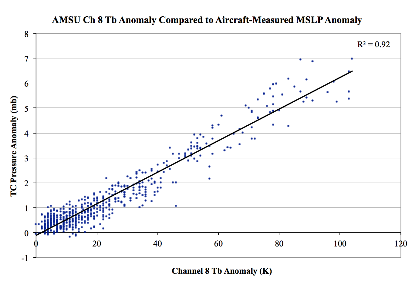
The CIMSS AMSU algorithm uses this relationship to estimate TC MSLP. In general during the early stages of TC development the associated warm core is located near channel 7. As the TC intensifies the warm core moves higher in the atmosphere closer to the mean location of channel 8. As the storm begins to move into higher latitudes and vertical wind shear increases the warm core maximum may move back lower into the atmosphere near channel 7 and then channel 6. The CIMSS AMSU algorithm weights the pressure anomaly contribution of each channel to get an estimate of MSLP. While warm anomalies often show up in the lower channels these channels tend to suffer from precipitation effects that reduces their effectiveness. Current research is addressing this issue (see below) and it is possible they can be used in the future. In the above image it is apparent that there is increased scatter in the brightness temperature relationship as intensity increases. This scatter has several sources including under-sampling by the AMSU instrument, precipitation contamination in the channel being used to produce the intensity estimate and positioning of the storm center in-between AMSU Fields of View. Each of these complications is addressed below:
Under-SamplingThe AMSU instrument employs a cross-track scanning strategy. As such the resolution of each of the 30 Fields Of View (FOV), or scenes, used by the instrument decreases with increasing scan angle. The CIMSS AMSU algorithm produces intensity estimates for AMSU-A FOV 3-28. A horizontal representation looks like the scan swath below.
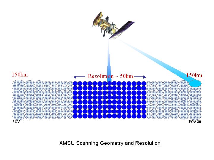
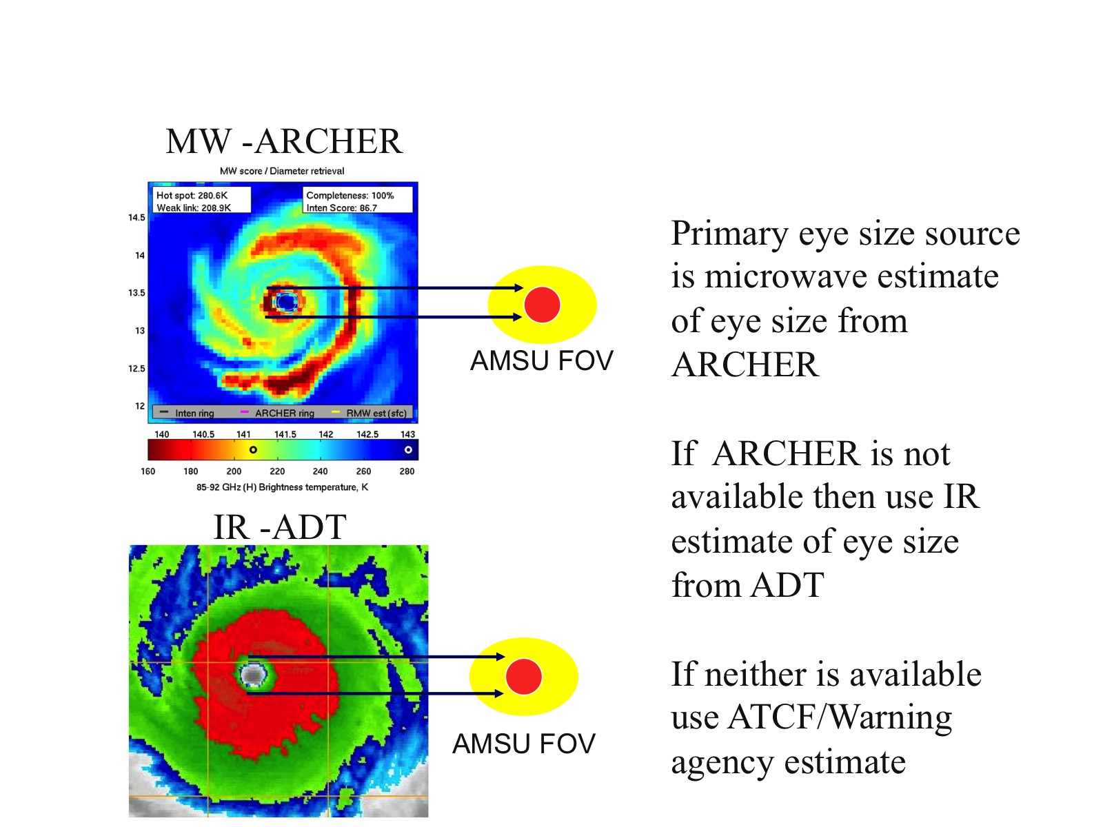
Much of the warming associated with a TC is concentrated in the eye region. The eye of a TC may be much less than the 150 km resolution of the near limb region of the scan swath. For example the eye of Hurricane Charley in 2004 was only about 8 km across. In these cases the warm anomaly signal will be signficantly under-sampled. To correct for this effect the cases used to develop the CIMSS AMSU algorithm were divided into 2 stratifications, well resolved and under-sampled. In order to determine whether or not a case falls into either category information regarding the eye size was needed. All cases for the 1998-2006 data sample were evaluated for eye size using available microwave, recconaisance obervations and IR imagery. These eye sizes were then compared to the FOV used to produce the intensity estimate for each AMSU pass. Cases in which the storm was well- resolved were then used to develop regression coefficients relating the brightness temperature anomalies to observed MSLP. These coefficients were then used to estimate the MSLP of the under-sampled cases. In nearly all the cases the estimate was substantially weak, in extreme cases by as much as 30 mb. These extreme cases were the result of a combination of very small eye size and poor scan geometry (FOV near the edge of the scan swath). A bias relationship was then developed for the under-sampled cases. The eye size / FOV resolution comparison explains about 50% of the observed error. When a storm is determined to be poorly sampled this bias is subtracted from the initial estimate. The method relies on accurate determination of the eye size. The operational algorithm gets the eye size from one of three sources. The CIMSS ARCHER algorithm objectively determines eye size from 85-92 GHz microwave imagery. If a microwave eye size is available within 3 hours of the AMSU estimate then that value is used. Otherwise if IR imagery is available and a clear well-defined eye is present then the eye size from the ADT is used. Finally if neither of these sources is available the RMW or eye size from the ATCF messages distributed by the operational TC forecast centers is used. There are times when the RMW does not accurately represent the storms core size. Storms undergoing Eyewall Replacement Cycles (ERC) often have more than one wind maxima. It is not known how much and at what point the outer convective ring becomes the dominant source of subsidence and when the inner ring no longer contributes. High level recconnaisance above 500 mb would be helpful in in understanding this process better.
More recent microwave sounders such as SSMIS and ATMS have improved resolution and resolve more of the TC warm core anomaly compated to AMSU. While eye size corrections are still needed the corrections tend to be smaller. Please see the CIMSS SSMIS and ATMS products page for additional information.
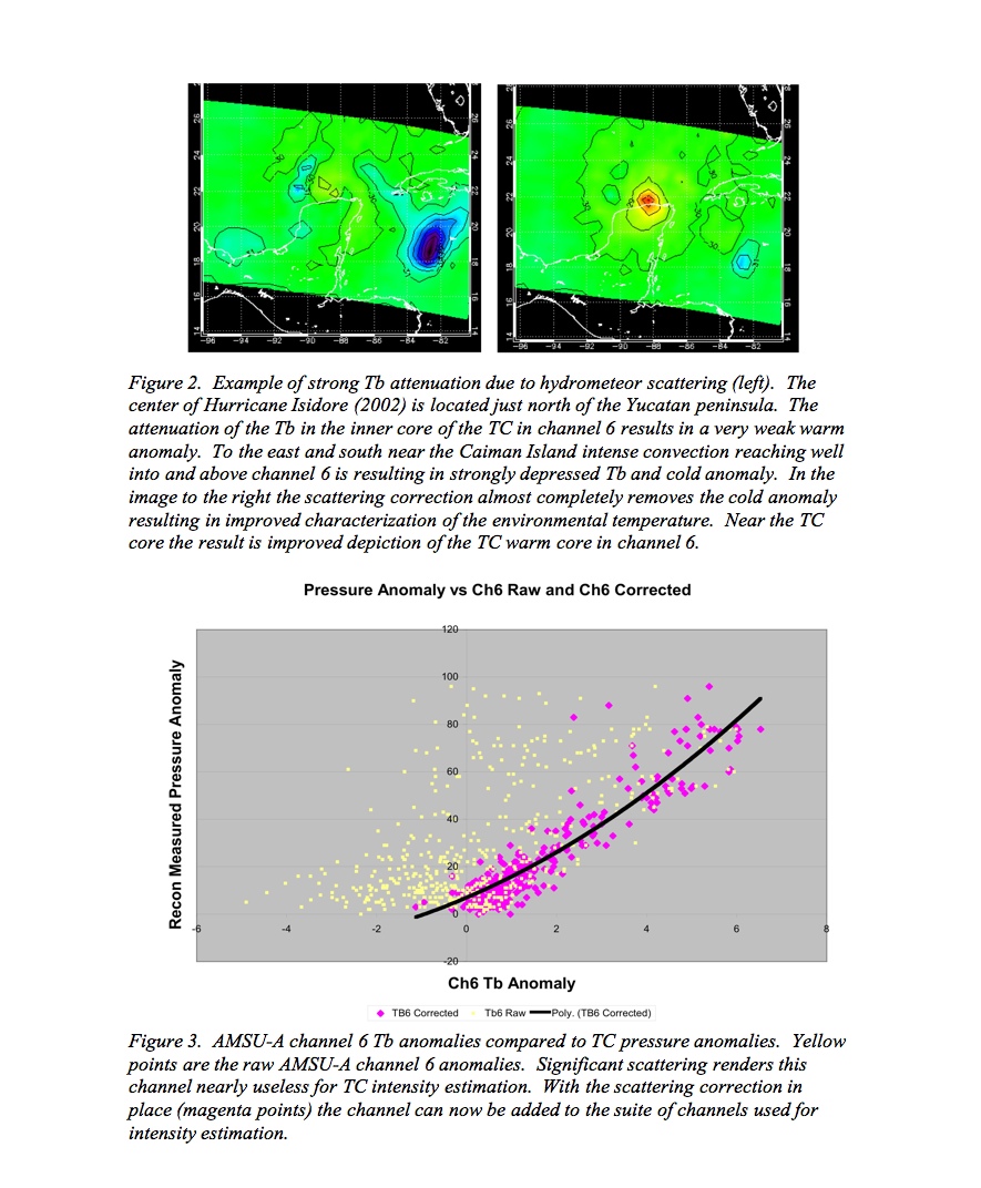
Hydrometeor Scattering and AttenuationChannels 7 and 8 are often high enough in the atmosphere to avoid the effects of precipitation. However, occasionally the convective towers associated with the TC and the associated scattering from hydrometeors may reach high enough to decrease the magnitude of the warm core signal. This is especially problematic when the TC is weak and the associated warm core is weak. In extreme cases the cooling effect of precipitation may completely mask the warm core signal and the result is a weak intensity estimate or no estimate at all. The example below shows a case for Tropical Depression 01W on January 11, 2002 where the effects of precipitation extend well into channel 8. The cooling is located very near the storm center making an intensity estimate difficult.
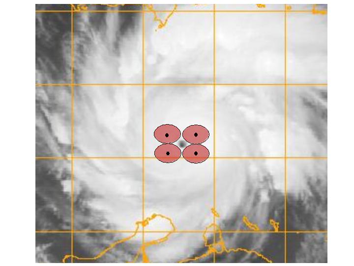
Another source of error for the algorithm is associated with storm position relative to the FOV used for the estimate. The initial
estimate of storm position is obtained from operational warnings and storm center fixes from the TC Forecast Centers. From the
initial fix a search is performed to check adjacent FOV's for the warmest pixel. However, given the instrument resolution it
is possible that the storm may fall in between FOV positions. If the storm center falls nearly equidistant from adjacent FOV
positions then the FOV will only sample the edge of the warm core and a weak estimate will result. This problem is aggravated
for cases when the eye is small. At the other extreme if the storm center is centered on the FOV position and the eye is large
then the estimate may be a 5-10 mb too deep since there is very little or no convection within the FOV to decrease the signal.
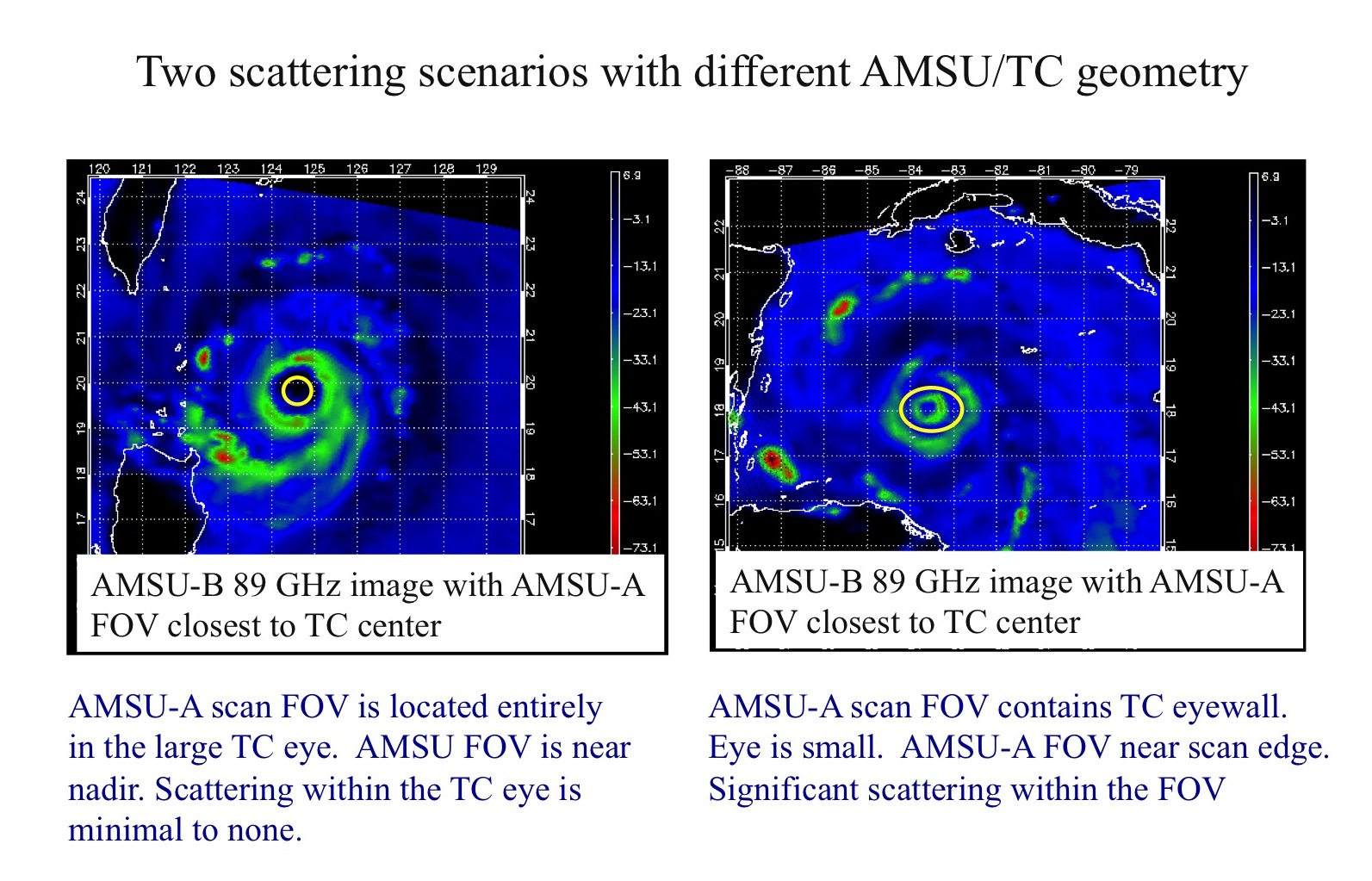
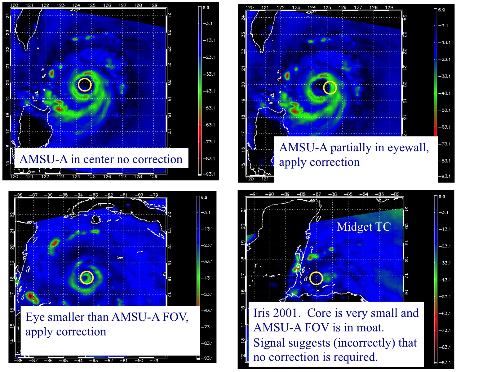
An objection measure of the amount of bracketing can be obtained by convolving the AMSU-B 89 GHz Tb to the AMSU-FOV used for the
intensity estimate. Cold AMSU-B Tb's indicate that the AMSU-A FOV is located at least partially within the TC eyewall while
warm AMSU-B Tb's indicate the liklihood that the AMSU-A FOV is located within the eye. Details on this bracketing factor
can be found in the most recent algorithm upgrade document (Word) here AMSU algorithm 2007
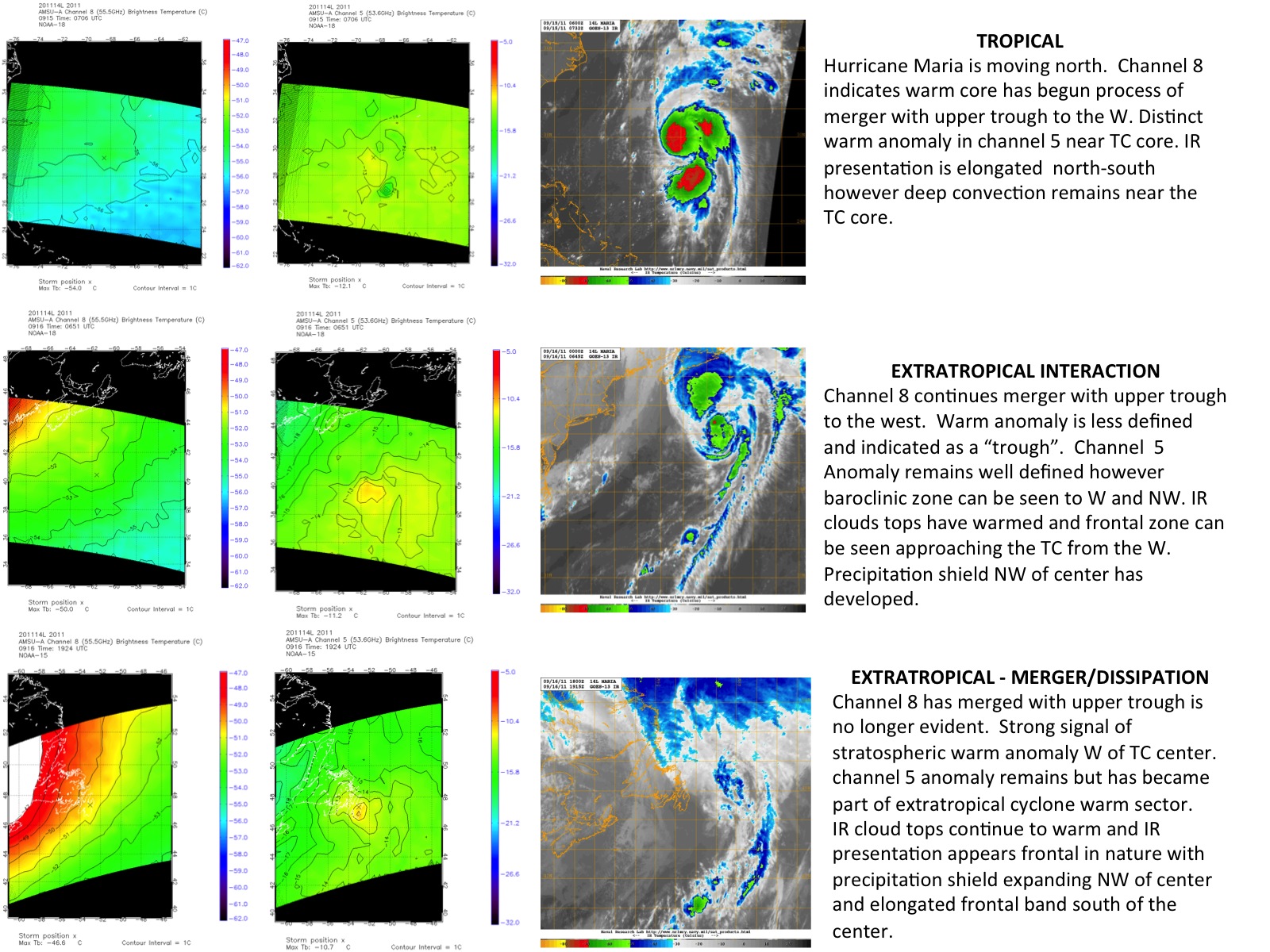
AMSU imagery can aid in the assesment of tropical and extra-tropical transitions. Cold low transition to a warm core system can at times be difficult to interpret since since the lowered tropopause and subsequent intrusion of warm stratospheric air in the upper AMSU channels can give the appearance of a "warm core". In these cases the transition to a TC or sub-tropical cyclone can often be seen in the lower AMSU channels first as convection builds in depth and coverage near the inner core of the cyclone and gradually warms the environment. A cold low "warm anomaly" signal may continue in the AMSU upper channels during this time. ET can occur through several pathways. A typical pathway is capture and merger of the TC with a pre-existing or developing bacroclinic system. This can often been seen starting in AMSU channel 8 as the upper tropospheric trough approaches from the west. The lowered toposphere and statospheric air intrusion will be depicted by a warm anomaly located somewhere to the southwest-northwest of the TC warm core. Increasing wind shear will general erode the TC upper warm core and the TC warm anomaly may dissapear from channel 8. The lower channels may continue to depict the TC warm core however the baroclinic system may become apparent in the lower AMSU channels west and north of the TC. Eventually the convection associated with the TC weakens substantially and the warm core will expand. The remnant warm core in the lower channels may merge with or become the warm sector of the extra-topical system.
The following results are from the 1999-2012 seasons. Validation consisted of recconnaisance observations within 3 hours of the AMSU estimate. Dvorak statistics were produced using an average of available Dvorak estimates from TAFB and SAB in Atlantic and Eastern Pacific or SAB and JTWC in the Western Pacific. In general the intensity algorithm performs best for estimating MSLP since the warm core anomaly measured by AMSU is directly related to the TC MSLP anomaly. A too strong bias can exist early in the TC stages of development and intensification stage (intensity less than 45 knots). While corrections are applied to account for eye size tropical cyclones with very small eyes may have a too weak bias. This bias is largest when the TC falls near the edge of the AMSU scan swath.